1.3 Format Cells – Number Tab – Intermediate Excel 2016

FIGURE 1

Right-button mouse click the cell and select Format Cells from the mouse shortcut menu (FIGURE 1).

FIGURE 2

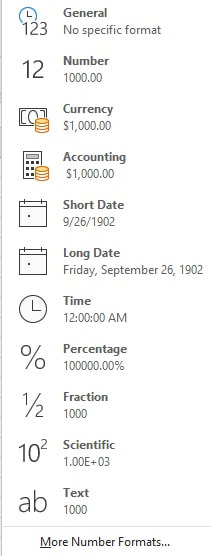FIGURE 3

Select downward pointing arrow in formatting window (shown in FIGURE 2) and select “More Number Formats” at the bottom of the drop-down menu (FIGURE 3).

General formatting is the default cell format (FIGURE 5). If you select a cell and go into Format Cells dialog box, you will observe the above, with General formatting highlighted. General formatting works well for many purposes. It does not allow you to add decimal places. It allows you to enter up to a 11-digit number.
The Sample area will show what your current active cell will display if a specific Category type is selected.

FIGURE 5

Number formatting allows you several display options (FIGURE 6). You can add decimal places. You can add decimal places, use 1000 separator (comma), and have negative numbers represented by a minus, in parenthesis, or in a red color.  Number formatting allows you to enter up to a 15-digit number.
The Sample area will show what your current active cell will display if a specific Category type is selected.

FIGURE 6

​Currency formatting is used for general monetary values (FIGURE 7). You can add decimal places, and have negative numbers represented by a minus, in parenthesis, or in a red color. You can also change country currency standard symbol. 
The Sample area will show what your current active cell will display if a specific Category type is selected.

FIGURE 7

​Accounting formatting lines up the currency symbols and decimal points in a column (FIGURE 8). It’s options include adding decimal places and changing country currency standard symbol.
The Sample area will show what your current active cell will display if a specific Category type is selected.

FIGURE 8

​Date formatting displays date and time serial numbers as date values (FIGURE 9). Date formats that begin with an asterisk respond to changes in regional date and time settings that are specified for the operating system. Formats without an asterisk are not affected by operating system settings. Options include location.
The Sample area will show what your current active cell will display if a specific Category type is selected.

FIGURE 9

​Time formatting displays date and time serial numbers as date values (FIGURE 10). Time formats that begin with an asterisk respond to changes in regional date and time settings that are specified for the operating system. Formats without an asterisk are not affected by operating system settings. The Sample area will show what your current active cell will display if a specific Category type is selected.

FIGURE 10

​Percentage formatting multiplies the cell value by 100 and displays the result with a percent symbol (FIGURE 11). If a cell has General formatting and you enter a number with a percent symbol, the cell formatting will automatically change to Percentage formatting. Options include changing decimal places.
The Sample area will show what your current active cell will display if a specific Category type is selected.

FIGURE 11

Fraction formatting allows you to enter a fraction with varying degrees of measurement (FIGURE 12). If you desire to enter a fraction with two digits such as 21/25, select the Type as Up to two digits. Applying Fraction formatting will also show a decimal as its fractional equivalent, i.e. .75 in the cell will display as 3/4.
The Sample area will show what your current active cell will display if a specific Category type is selected.

FIGURE 12

Scientific formatting allows a number to be represented in exponential notation, replacing part of the number with E + n, where E (stands for Exponent) multiplies the preceding number by 10 to the nth power (FIGURE 13). Options include changing decimal places. If you have General formatting applied to a cell, and enter a 12-digit number, that number will be represented in a Scientific Notation format, although the cell formatting remains as General. The Sample area will show what your current active cell will display if a specific Category type is selected.

FIGURE 13

​Text formatting treats the content of the cell as text and displays the content exactily as you type it, even when you enter numbers (FIGURE 14). If you need to enter a number greater than 15 digits and have the number displayed as such, Text formatting will allow you to do it.
The Sample area will show what your current active cell will display if a specific Category type is selected.

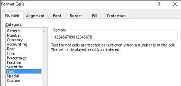FIGURE 14

​Special formatting allows you to display a number as a postal code (ZIP Code), phone number, or Social Security number (FIGURE 15).
The Sample area will show what your current active cell will display if a specific Category type is selected.

FIGURE 15

Custom number formatting allows you to modify a copy of an existing number format code (FIGURE 16). Once created, it will be added to this Type listing. The Sample area will show what your current active cell will display if a specific Category type is selected.

​Create a custom number format

1. In the Category box, click Custom.
2. In the Type list, select the number format that you want to customize. The number format that you select appears in the Type box above the Type list.

 Note   When you select a built-in number format in the Type list, Excel creates a copy of that number format that you can then customize. The original number format in the Type list cannot be changed or deleted.

In the Type box, make the necessary changes to the selected number format.A number format can have up to four sections of code, separated by semicolons. These code sections define the format for positive numbers, negative numbers, zero values, and text, in that order.
<POSITIVE>;<NEGATIVE>;<ZERO>;<TEXT>
 
For example, you can use these code sections to create the following custom format:
[Blue]#,##0.00_);[Red](#,##0.00);0.00;”sales “@

​One great use of using custom numbers is preventing Excel from clipping off the leading zero of a number. Enter a series of zeros up to the number of number digits.

​Custom numbers can be saved to a workbook.  A custom number format is stored in the workbook in which it was created but will not be available in any other workbooks. To use a custom format in a new workbook, you can save the current workbook as an Excel template that you can use as the basis for the new workbook (FIGURE 17).

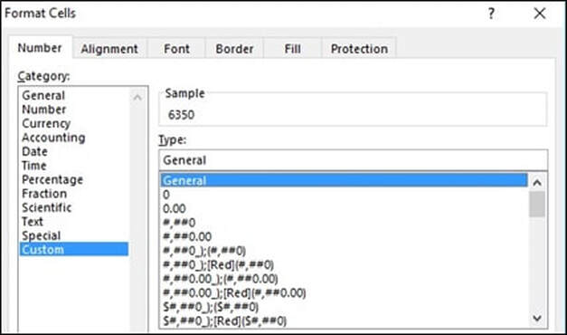FIGURE 16

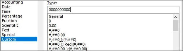FIGURE 17