Your cart is currently empty!
2.3 Practice Exercise 4 – Organize and Clean Data in the CUSTOMERS Table
|
STEP 1: Select the CUSTOMERS table (FIGURE 1). We will work on cleaning the data.
|

FIGURE 1
|
STEP 2: Let’s begin cleaning our data by eliminating the top header row.
Ensure you have a cell in the CUSTOMERS table as the active cell. In the Ribbon contextual tab, Table Design, uncheck the box “Header Row” (FIGURE 2). |
 FIGURE 2
|
STEP 3: The header row with the temporary header field labels has been removed from the CUSTOMERS table (FIGURE 3).

FIGURE 3
|
STEP 4A: We will delete Row 1 since it is empty. Select the Row 1 header to highlight Row 1.
STEP 4B: Right-button mouse click Row 1 and select “Delete” from menu (FIGURE 4). |
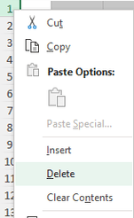 FIGURE 4
|
STEP 4C: We have removed Row 1 (FIGURE 5)

FIGURE 5
STEP 5A: Make cell A1 the active cell.
STEP 5B: Select keys CTRL + SHIFT + Down Arrow to highlight Column A cells A1 through A134.
STEP 5C: Scroll down to cell A134, place mouse on edge of highlighted cell and move mouse until it turns into a 4-headed arrow. Click and drag Column A down one row with the mouse.
STEP 5D: ID 1 should now be in Row 2, ID 2 should be in Row 3 and so on (FIGURE 6).

FIGURE 6
|
STEP 6A: Remove Column F by selecting the Column F header to highlight Column F.
STEP 6B: Right-button mouse click Column F and select “Delete” from menu. (FIGURE 7). |
 FIGURE 7
|
STEP 6C: Column F has been removed (FIGURE 8).

FIGURE 8
STEP 7: We have missing column headers in cells A1 and B1. Let’s add “ID” into cell A1 and “CustomerID” into cell B1 (FIGURE 9).

FIGURE 9
|
STEP 8A: Let’s check and remove any duplicates.
STEP 8B: Select the Data tab on the Ribbon. STEP 8C: From the Ribbon section, “Data Tools” select the icon, “Remove Duplicates” (FIGURE 10). |
 FIGURE 10
|
|
STEP 9A: The Remove Duplicates dialog box appears. Check the box, “My data has headers” (FIGURE 11).
STEP 9B: Ensure all boxes are checked for all fields. Select OK button. |
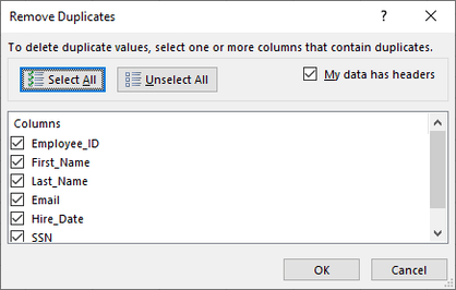 FIGURE 11
|
|
STEP 9C: “No duplicate values found” dialog box appears. Select OK button (FIGURE 12).
|
 FIGURE 12
|
|
STEP 10A: Make cell address K3 the active cell (FIGURE 13).
STEP 10B: Enter: =LEFT(J3,5) STEP 10C: Note: the J3 can be entered by selecting cell address J3 with mouse Press Enter key. |
 FIGURE 13
|
|
STEP 11: We get the data we desired; we now have the number reproduced, without the hyphen and last 4 zip code digits (FIGURE 14).
All values in column lose the last 4 digits and hyphen of zip code |
 FIGURE 14
|
|
STEP 12A: Make cell L3 active (FIGURE 15).
STEP 12B: Press CTRL + Shift + down arrow. All data in Column L is highlighted. STEP 12C: Right-button mouse click the highlighted data and select Copy STEP 12D: Make cell K3 active. Press CTRL + Shift + down arrow. All data in Column K is highlighted. STEP 12E: Right-button mouse click the highlighted data and select Paste – Values. |
 FIGURE 15
|
|
STEP 13: Now we can remove Column L. Select Column L header; right-button mouse click data and select Delete from mouse menu (FIGURE 16).
|
 FIGURE 16
|
|
END OF PRACTICE EXERCISE 4
|